Mechanics in jax-morph

A tour of the Phase 2 mechanics (jax_morph.physics), the physical layer built on the core's step contract. Each is a step or a reusable potential:

• Morse - a soft-matter pair potential with a well at the contact distance sigma = r_i + r_j and a smooth, size-relative cutoff. It is a PairwisePotential, so it hands you total_energy, forces, and per-cell virial_pressure for free.
• MechanicalRelaxation - a quasistatic step that relaxes positions to mechanical equilibrium with FIRE, differentiated by the implicit function theorem (the gradient is the equilibrium sensitivity, not the solver path).
• BrownianDynamics - a dynamic, stochastic step: one Euler-Maruyama step of overdamped Langevin dynamics, both pathwise-differentiable and scorable (transition_logp).
• VirialStress - a quasistatic step exposing the per-cell virial pressure as a stress sensing field.
• SaturatingCellGrowth - a dynamic step: saturating radius growth toward max_radius at a per-cell rate, so the rate (and its gradient) can come from an upstream controller.

Everything here is differentiable. We plot the simulations and the gradients they expose.

import jax
import jax.numpy as jnp

# The library is written for float64; enable it before anything touches JAX.
jax.config.update('jax_enable_x64', True)

import numpy as np
import equinox as eqx
import matplotlib.pyplot as plt

%matplotlib inline

import jax_morph as jxm
from jax_morph.physics.mechanics import (
    Morse,
    MechanicalRelaxation,
    relax_equilibrium,
    BrownianDynamics,
    VirialStress,
)
from jax_morph.physics.growth import SaturatingCellGrowth

key = jax.random.PRNGKey(0)
print('jax-morph', jxm.__version__)

jax-morph 0.4.0

A tiny helper to build a live cluster from an array of positions. build_state_from_model generates the typed state class for whatever model (or bare potential) we hand it; we then seed the first n slots alive with the given positions and radii. (The library deliberately ships no seeding helper - the initial condition is the simulation's job.)

class _Bare:
    # A model with no declared fields: the state then carries only the base fields (position, radius,
    # celltype, alive, t). Used when we only need a state to evaluate a potential on.
    def state_requires(self):
        return ()


def make_state(model, positions, *, radius=0.5, space=None):
    positions = jnp.asarray(positions, dtype=float)
    n, dim = positions.shape
    State = jxm.build_state_from_model(model)
    s = State.init_empty(capacity=n, n_space_dim=dim, n_types=1, space=space)
    return s.update(
        alive=s.alive.at[:n].set(True),
        radius=s.radius.at[:n].set(radius),
        position=s.position.at[:n].set(positions),
        celltype=s.celltype.at[:n, 0].set(1.0),  # one cell type (one-hot)
    )

def shared_limits(s, pad=0.4):
    # Common, generous axis limits taken from a state's live cells, so panels sharing them are drawn
    # to the same scale and relative cluster sizes stay visible.
    pos = np.asarray(s.position)[np.asarray(s.alive).astype(bool)]
    m = float(np.asarray(s.radius).max()) + pad
    return (
        (pos[:, 0].min() - m, pos[:, 0].max() + m),
        (pos[:, 1].min() - m, pos[:, 1].max() + m),
    )

1. The Morse pair potential

For a pair at separation r with contact distance sigma = r_i + r_j, the Morse energy is

U(r) = epsilon * ((1 - exp(-alpha (r - sigma)))^2 - 1) * S(r)

a well of depth epsilon and width set by alpha, minimized exactly at r = sigma. S(r) is a smooth multiplicative cutoff (the jax-md form) that switches the interaction off between r_onset_frac * sigma and r_cutoff_frac * sigma, so the cutoff is size-relative and the energy stays continuous. Let's plot the energy and the pair force F = -U'(r) for a unit contact distance.

pot = Morse()  # defaults: epsilon=3.0, alpha=2.8, r_onset_frac=1.5, r_cutoff_frac=2.5
sigma, eps, alpha = 1.0, pot.epsilon, pot.alpha

r = jnp.linspace(0.55, 3.0, 500)
U = jax.vmap(lambda rr: pot.pair_energy(rr, sigma, eps, alpha))(r)
F = -jax.vmap(jax.grad(lambda rr: pot.pair_energy(rr, sigma, eps, alpha)))(r)

fig, (a0, a1) = plt.subplots(1, 2, figsize=(11, 4))
a0.plot(r, U, color='tab:blue')
a0.axhline(0, color='0.7', lw=0.8)
a0.axvline(sigma, color='tab:green', ls=':', label='sigma (contact / well)')
a0.axvline(pot.r_onset_frac * sigma, color='tab:orange', ls='--', label='cutoff onset')
a0.axvline(pot.r_cutoff_frac * sigma, color='tab:red', ls='--', label='cutoff end')
a0.set(xlabel='separation r', ylabel='U(r)', title='Morse energy')
a0.legend(fontsize=8)

a1.plot(r, F, color='tab:purple')
a1.axhline(0, color='0.7', lw=0.8)
a1.axvline(sigma, color='tab:green', ls=':')
a1.set(xlabel='separation r', ylabel='F(r) = -U\'(r)', title='Morse pair force')
a1.annotate('repulsion (F>0)', (0.62, F[0] * 0.5), fontsize=8)
a1.annotate('attraction (F<0)', (1.35, F.min() * 0.6), fontsize=8)
fig.tight_layout()
plt.show()

print('well minimum near r =', float(r[jnp.argmin(U)]), '(sigma =', sigma, ')')

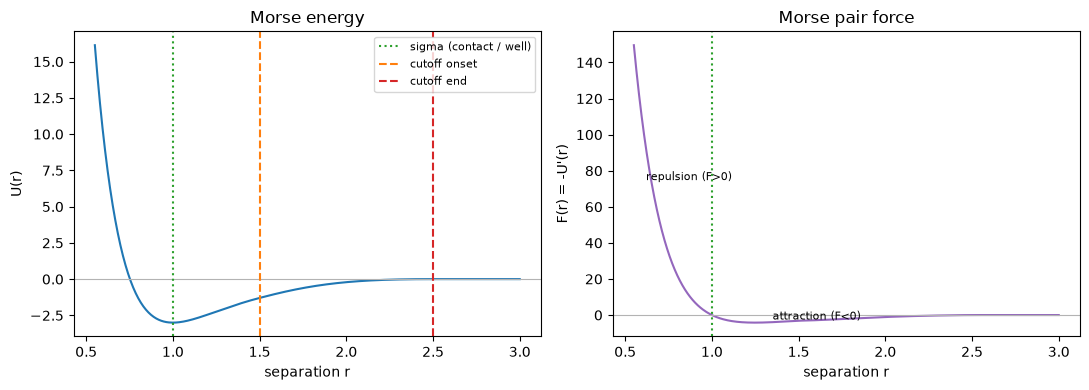
well minimum near r = 1.0017034068136272 (sigma = 1.0 )

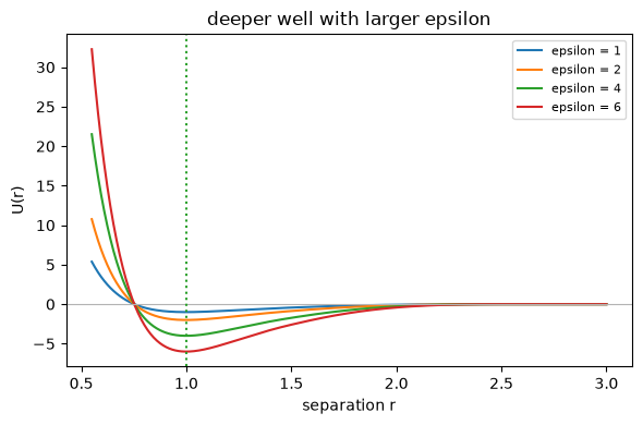
Couplings: shared or per-cell. Each coupling (epsilon, alpha) is either a shared scalar (a Python float is frozen; a jax.Array is traced and optimizable) or a per-cell value read from a state field - pass a StateFieldSpec and the pair value is the arithmetic mean of the two cells' values (mix). A per-cell coupling can be a fixed initial condition or, in a full model, written each step by an upstream controller, so type-dependent interactions come from writing the field from celltype (there is no separate per-type matrix). First, the shared-scalar case: sweep the well depth epsilon and watch the well deepen.

fig, ax = plt.subplots(figsize=(6, 4))
for e in [1.0, 2.0, 4.0, 6.0]:
    p = Morse(epsilon=e)
    Ue = jax.vmap(lambda rr: p.pair_energy(rr, sigma, e, p.alpha))(r)
    ax.plot(r, Ue, label=f'epsilon = {e:g}')
ax.axhline(0, color='0.7', lw=0.8)
ax.axvline(sigma, color='tab:green', ls=':')
ax.set(xlabel='separation r', ylabel='U(r)', title='deeper well with larger epsilon')
ax.legend(fontsize=8)
fig.tight_layout()
plt.show()

Now a per-cell coupling: give epsilon a StateFieldSpec so it is read from the state. The owning step surfaces that read, so build_state_from_model allocates the field; here two cells get different well depths and the pair feels their arithmetic mean.

adhesion = jxm.StateFieldSpec('adhesion')          # a per-cell field the potential reads epsilon from
pot_pc = Morse(epsilon=adhesion)
model_pc = jxm.Model([MechanicalRelaxation(pot_pc, max_steps=1, f_tol=1e-6)])  # any owner surfaces the read
State_pc = jxm.build_state_from_model(model_pc)     # the synthesized schema now carries `adhesion`

s_pc = State_pc.init_empty(capacity=2, n_space_dim=2, n_types=1)
s_pc = s_pc.update(
    alive=s_pc.alive.at[:2].set(True),
    radius=s_pc.radius.at[:2].set(0.5),
    position=jnp.array([[0.0, 0.0], [1.0, 0.0]]),   # at contact (r = sigma = 1.0)
    adhesion=s_pc.adhesion.at[:2].set(jnp.array([2.0, 6.0])),  # different per-cell well depths
)
well = -float(pot_pc.total_energy(s_pc.position, s_pc))
print('per-cell epsilons 2.0 and 6.0 -> pair well depth (arithmetic mean):', well, '  (= (2 + 6) / 2)')
print('the potential surfaces its field read:', [s.name for s in pot_pc.state_reads()])

per-cell epsilons 2.0 and 6.0 -> pair well depth (arithmetic mean): 4.0   (= (2 + 6) / 2)
the potential surfaces its field read: ['adhesion']

Virial pressure (per-cell stress)

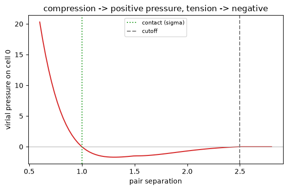
Because Morse is a PairwisePotential, it also gives a per-cell virial pressure p_i = -(1 / (2 d V_i)) sum_j r_ij U'(r_ij) (Irving-Kirkwood bond split; the sign makes compression positive). We sweep a two-cell separation and read the pressure on one cell: it is large and positive when the cells are pushed inside contact (r < sigma), passes through zero at the force-free contact, and vanishes once the pair is beyond the cutoff.

dists = np.linspace(0.6, 2.8, 80)
press = np.array([
    float(pot.virial_pressure(make_state(_Bare(), jnp.array([[0.0, 0.0], [d, 0.0]])))[0])
    for d in dists
])

fig, ax = plt.subplots(figsize=(6, 4))
ax.plot(dists, press, color='tab:red')
ax.axhline(0, color='0.7', lw=0.8)
ax.axvline(sigma, color='tab:green', ls=':', label='contact (sigma)')
ax.axvline(pot.r_cutoff_frac * sigma, color='0.5', ls='--', label='cutoff')
ax.set(xlabel='pair separation', ylabel='virial pressure on cell 0',
       title='compression -> positive pressure, tension -> negative')
ax.legend(fontsize=8)
fig.tight_layout()
plt.show()

2. Mechanical relaxation (FIRE + implicit-diff)

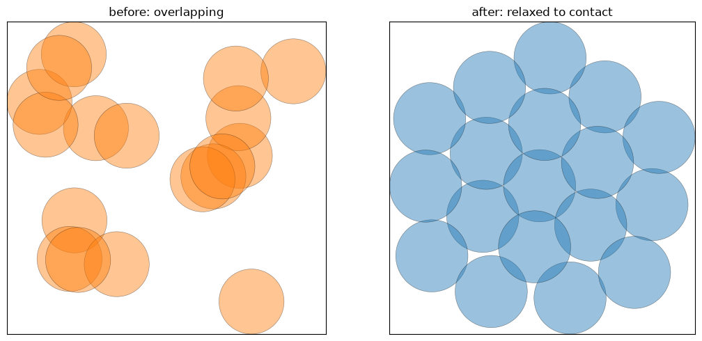
MechanicalRelaxation is a quasistatic step: each macro-step it drives the positions to a genuine force equilibrium |grad U| <= f_tol with the FIRE minimizer. Let's start from a messy, overlapping blob of cells and relax it - the overlaps (deep in the repulsive core) push apart until neighbours sit at their contact distance.

n = 18
blob = 1.4 * jax.random.normal(jax.random.PRNGKey(3), (n, 2))  # a compact, overlapping cluster
relax = MechanicalRelaxation(Morse(), max_steps=1500, f_tol=1e-5)

s0 = make_state(jxm.Model([relax]), blob, radius=0.5)
s1 = relax(s0, dt=1.0, key=None)  # a quasistatic step: ignores dt/key, returns the relaxed state

pot = Morse()
print('max |force| before relax:', float(jnp.max(jnp.abs(pot.forces(s0)))))
print('max |force| after  relax:', float(jnp.max(jnp.abs(pot.forces(s1)))))

fig, (a0, a1) = plt.subplots(1, 2, figsize=(11, 5))
jxm.viz.draw(s0, ax=a0, color='tab:orange', alpha=0.45, title='before: overlapping')
jxm.viz.draw(s1, ax=a1, color='tab:blue', alpha=0.45, title='after: relaxed to contact')
fig.tight_layout()
plt.show()

max |force| before relax: 2015.7309247507778
max |force| after  relax: 8.619358744105243e-06

The gradient is an equilibrium sensitivity

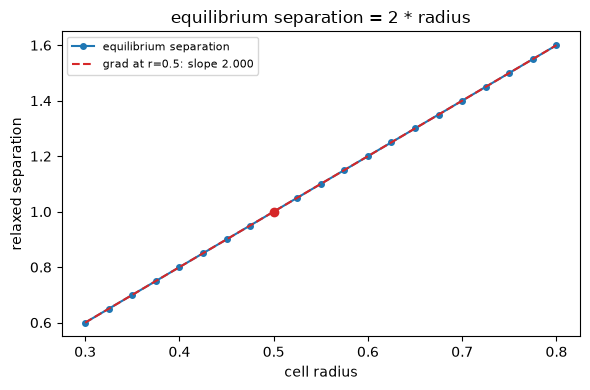
The point of the implicit-diff relaxation is that d(equilibrium) / d(parameters) is the sensitivity of the converged state, independent of the solver's path. The cleanest check: a two-cell system relaxes to separation sigma = 2 * radius, so d(separation) / d(radius) must be exactly 2 - and jax.grad through the whole FIRE solve recovers it. We sweep the radius to draw the equilibrium curve, then overlay the tangent that jax.grad returns at radius = 0.5.

relax2 = MechanicalRelaxation(Morse(), max_steps=1500, f_tol=1e-9)


def separation(radius):
    s = make_state(jxm.Model([relax2]), jnp.array([[0.0, 0.0], [1.0, 0.0]]), radius=radius)
    s2 = relax2(s, dt=1.0, key=None)
    return jnp.linalg.norm(s2.position[0] - s2.position[1])


radii = np.linspace(0.3, 0.8, 21)
seps = np.array([float(separation(r)) for r in radii])

r0 = 0.5
g = float(jax.grad(separation)(r0))  # implicit-function-theorem gradient through the equilibrium
s0_val = float(separation(r0))
print('d(separation)/d(radius) via implicit diff:', g, '   (analytic: 2.0)')

fig, ax = plt.subplots(figsize=(6, 4))
ax.plot(radii, seps, 'o-', ms=4, label='equilibrium separation')
tang = s0_val + g * (radii - r0)
ax.plot(radii, tang, '--', color='tab:red', label=f'grad at r=0.5: slope {g:.3f}')
ax.scatter([r0], [s0_val], color='tab:red', zorder=5)
ax.set(xlabel='cell radius', ylabel='relaxed separation', title='equilibrium separation = 2 * radius')
ax.legend(fontsize=8)
fig.tight_layout()
plt.show()

d(separation)/d(radius) via implicit diff: 1.999999978741497    (analytic: 2.0)

3. Brownian dynamics

BrownianDynamics is a dynamic, stochastic step: one Euler-Maruyama step of overdamped Langevin dynamics,

dx = dt * (-grad U / gamma) + sqrt(2 kT dt / gamma) * xi,   xi ~ N(0, I)

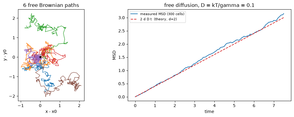
a deterministic drift down the potential plus Gaussian noise. simulate scans it to physical time. First, a free-diffusion check: far-apart cells (no force) should spread as MSD(t) = 2 d D t with the Einstein diffusivity D = kT / gamma. We run 300 non-interacting cells and average.

pot = Morse()
gamma, kT = 1.0, 0.1
D = kT / gamma
bd = BrownianDynamics(pot, n_space_dim=2, gamma=gamma, kT=kT)
model = jxm.Model([bd])

# 300 cells on a wide grid (spacing 50 >> cutoff): they never interact -> pure free diffusion.
side = 20
xs, ys = np.meshgrid(np.arange(side), np.arange(side))
grid = 50.0 * np.stack([xs.ravel(), ys.ravel()], axis=1)[:300].astype(float)
s_free = make_state(model, grid, radius=0.5)

dt, n_steps = 0.05, 150
traj = jxm.simulate(model, s_free, n_steps=n_steps, dt=dt, key=key, history=True)

pos0 = np.asarray(s_free.position)
posT = np.asarray(traj.position)                       # (n_steps + 1, n_cells, 2)
msd = ((posT - pos0[None]) ** 2).sum(-1).mean(1)       # includes the zero-displacement initial frame
t = np.asarray(traj.t)

fig, (a0, a1) = plt.subplots(1, 2, figsize=(11, 4))
for i in range(6):  # a handful of individual Brownian paths (recentred to their start)
    p = posT[:, i, :] - pos0[i]
    a0.plot(p[:, 0], p[:, 1], lw=1)
a0.scatter([0], [0], color='k', s=15, zorder=5)
a0.set_aspect('equal')
a0.set(xlabel='x - x0', ylabel='y - y0', title='6 free Brownian paths')

a1.plot(t, msd, label='measured MSD (300 cells)')
a1.plot(t, 2 * 2 * D * t, '--', color='tab:red', label='2 d D t  (theory, d=2)')
a1.set(xlabel='time', ylabel='MSD', title=f'free diffusion, D = kT/gamma = {D:g}')
a1.legend(fontsize=8)
fig.tight_layout()
plt.show()

Scoring a transition: the score-function gradient

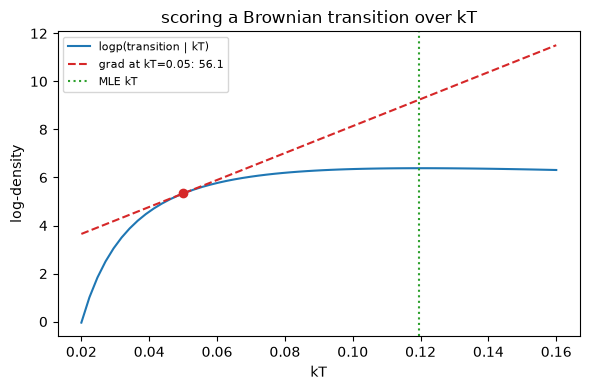
Brownian is a StochasticStep, so a transition (s_t, s_{t+1}) can be scored: transition_logp is the Gaussian log-density of the recorded displacement under the transition kernel, with parameters recomputed live. That makes kT, gamma, and the potential's parameters learnable from observed motion (MLE). A reparameterized step defaults to the pathwise estimator (next section), so we opt into scoring it explicitly with score='all'. We take one recorded transition of an interacting pair, then sweep kT in the scorer: the log-density peaks at the kT that best explains the displacement, and jax.grad gives the exact score at any point.

pair = make_state(jxm.Model([BrownianDynamics(pot, n_space_dim=2, kT=0.05)]),
                  jnp.array([[0.0, 0.0], [1.2, 0.0]]), radius=0.5)
m_sample = jxm.Model([BrownianDynamics(pot, n_space_dim=2, gamma=1.0, kT=0.05)])
pair_next = m_sample(pair, dt=0.01, key=key)  # sample + record the displacement into the trace


@jax.jit
def logp_of_kT(kt):  # kt a traced 0-d array -> compiled once, reused across the sweep
    m = jxm.Model([BrownianDynamics(pot, n_space_dim=2, gamma=1.0, kT=kt)])
    return jxm.transition_logp(m, pair, pair_next, 0.01, score='all')  # opt in: Brownian is pathwise by default


grad_logp = jax.jit(jax.grad(logp_of_kT))

kts = np.linspace(0.02, 0.16, 60)
lps = np.array([float(logp_of_kT(jnp.array(k))) for k in kts])

k0 = 0.05
g0 = float(grad_logp(jnp.array(k0)))
l0 = float(logp_of_kT(jnp.array(k0)))
print('d logp / d kT at kT=0.05:', g0)

fig, ax = plt.subplots(figsize=(6, 4))
ax.plot(kts, lps, label='logp(transition | kT)')
ax.plot(kts, l0 + g0 * (kts - k0), '--', color='tab:red', label=f'grad at kT=0.05: {g0:.1f}')
ax.axvline(kts[np.argmax(lps)], color='tab:green', ls=':', label='MLE kT')
ax.scatter([k0], [l0], color='tab:red', zorder=5)
ax.set(xlabel='kT', ylabel='log-density', title='scoring a Brownian transition over kT')
ax.legend(fontsize=8)
fig.tight_layout()
plt.show()

d logp / d kT at kT=0.05: 56.11847116902588

The other estimator: a pathwise gradient through simulate

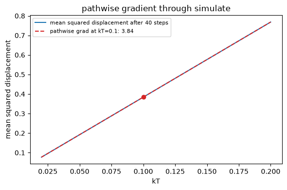
Because the noise is reparameterized (dx = mean + std * xi with xi frozen), the forward rollout is also pathwise-differentiable: we can differentiate a whole simulated trajectory with respect to kT directly, no scoring involved. Here the objective is the mean squared displacement of a free cloud after several steps; its value grows linearly with kT (variance scales with kT) and jax.grad returns the matching slope.

cloud = make_state(model, 50.0 * np.stack(np.meshgrid(np.arange(8), np.arange(8)), -1).reshape(-1, 2),
                   radius=0.5)


@jax.jit
def spread(kt):
    m = jxm.Model([BrownianDynamics(pot, n_space_dim=2, gamma=1.0, kT=kt)])
    final = jxm.simulate(m, cloud, n_steps=40, dt=0.02, key=key)
    a = cloud.alive.astype(final.position.dtype)[:, None]
    disp2 = ((final.position - cloud.position) ** 2 * a).sum()
    return disp2 / a.sum()


grad_spread = jax.jit(jax.grad(spread))

kts = np.linspace(0.02, 0.2, 60)
vals = np.array([float(spread(jnp.array(k))) for k in kts])
k0 = 0.1
g0 = float(grad_spread(jnp.array(k0)))
v0 = float(spread(jnp.array(k0)))
print('pathwise d(spread) / d(kT) at kT=0.1:', g0)

fig, ax = plt.subplots(figsize=(6, 4))
ax.plot(kts, vals, label='mean squared displacement after 40 steps')
ax.plot(kts, v0 + g0 * (kts - k0), '--', color='tab:red', label=f'pathwise grad at kT=0.1: {g0:.2f}')
ax.scatter([k0], [v0], color='tab:red', zorder=5)
ax.set(xlabel='kT', ylabel='mean squared displacement', title='pathwise gradient through simulate')
ax.legend(fontsize=8)
fig.tight_layout()
plt.show()

pathwise d(spread) / d(kT) at kT=0.1: 3.841777859207043

Drift + noise: aggregation

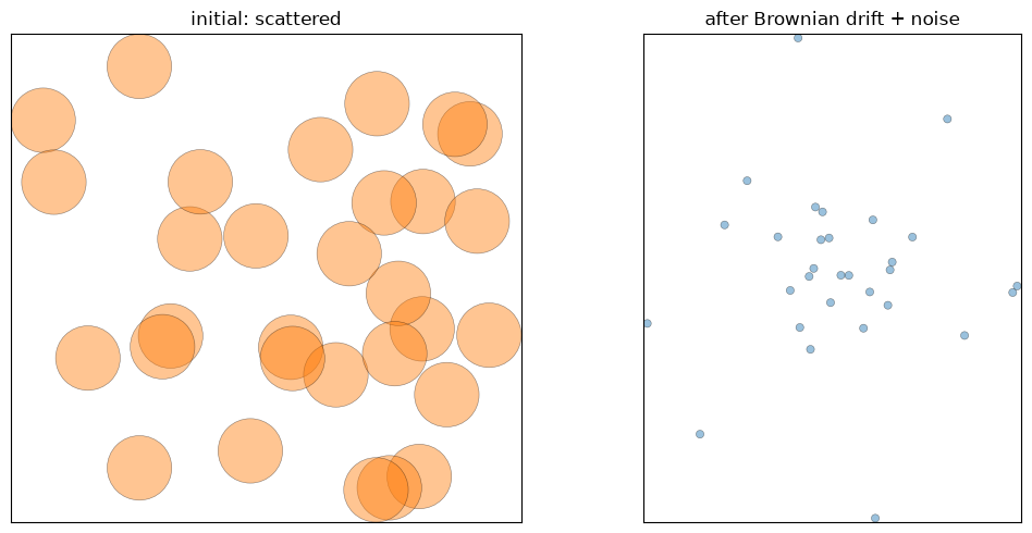
Put the two ingredients together at low temperature: the Morse drift pulls neighbours within the cutoff into contact while the noise lets the cluster rearrange. Starting from cells scattered across a few interaction lengths, a Brownian rollout condenses them into a packed aggregate.

bd_cold = BrownianDynamics(Morse(), n_space_dim=2, gamma=1.0, kT=0.02)
model_cold = jxm.Model([bd_cold])

n = 30
start = jax.random.uniform(jax.random.PRNGKey(7), (n, 2), minval=0.0, maxval=7.0)
s_start = make_state(model_cold, start, radius=0.5)
s_end = jxm.simulate(model_cold, s_start, n_steps=600, dt=0.02, key=jax.random.PRNGKey(8))

fig, (a0, a1) = plt.subplots(1, 2, figsize=(11, 5))
jxm.viz.draw(s_start, ax=a0, color='tab:orange', alpha=0.45, title='initial: scattered')
jxm.viz.draw(s_end, ax=a1, color='tab:blue', alpha=0.45, title='after Brownian drift + noise')
fig.tight_layout()
plt.show()

4. Virial stress (a per-cell sensing input)

VirialStress is a quasistatic step that writes each cell's virial pressure (from PairwisePotential.virial_pressure) into a stress field - a mechanical-load signal a control step can read. We compress a packed disk of cells (grid spacing 0.75, well inside the contact distance sigma = 1.0, so every cell is squeezed by its nearest neighbours) and colour each cell by its stress. The peak is not at the centre but in a sub-surface ring: every interior cell shares the same compressed nearest-neighbour core (the same positive, compressive contribution), but the attractive outer shell - which pulls the net pressure back down - is complete only deep in the bulk. A cell one shell below the free surface has lost part of that attractive shell, so it carries more pressure than the fully-embedded centre; the outermost cells then drop off as they shed compressed neighbours too.

spacing = 0.75
g = np.arange(-4, 5) * spacing
gx, gy = np.meshgrid(g, g)
pts = np.stack([gx.ravel(), gy.ravel()], axis=1)
pts = pts[np.linalg.norm(pts, axis=1) <= 3.6 * spacing]  # keep a rough disk

vs_model = jxm.Model([VirialStress(Morse())])
s_stress = vs_model(make_state(vs_model, pts, radius=0.5), dt=1.0, key=key)  # writes .stress

fig, ax = plt.subplots(figsize=(6, 5))
jxm.viz.draw(s_stress, ax=ax, color_by=s_stress.stress, cmap='Reds', alpha=0.95,
             title='per-cell virial stress (compressed disk)')
fig.axes[-1].set_ylabel('stress (pressure)')
fig.tight_layout()
plt.show()

# the maximum is a sub-surface ring, not the centre: same compressed core, but a thinner attractive
# shell (fewer outer neighbours pulling the pressure back down) than the fully-embedded centre cell.
radial = np.linalg.norm(pts, axis=1)
stress = np.asarray(s_stress.stress)
center_i, peak_i, edge_i = int(np.argmin(radial)), int(np.argmax(stress)), int(np.argmax(radial))
print(f'stress: centre {stress[center_i]:+.2f}'
      f'  |  peak ring (r={radial[peak_i]:.2f}) {stress[peak_i]:+.2f}'
      f'  |  outer edge {stress[edge_i]:+.2f}   (compression -> positive)')

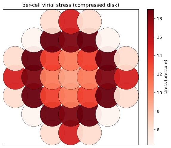
stress: centre +9.25  |  peak ring (r=1.68) +19.01  |  outer edge +6.34   (compression -> positive)

5. Saturating cell growth

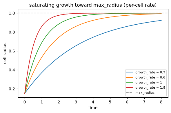
SaturatingCellGrowth is a dynamic step with a saturating (von Bertalanffy) law dr/dt = growth_rate * (1 - r / max_radius), integrated exactly (not forward Euler) so it stays stable for any dt. The rate is a per-cell state field (growth_rate), not a module parameter - so it can be a fixed initial condition or, in a full model, an upstream controller's output. Each cell approaches the shared max_radius, faster or slower according to its own rate.

model = jxm.Model([SaturatingCellGrowth(max_radius=1.0)])
State = jxm.build_state_from_model(model)
rates = [0.3, 0.6, 1.0, 1.8]

s = State.init_empty(capacity=len(rates), n_space_dim=2, n_types=1)
s = s.update(
    alive=s.alive.at[:].set(True),
    radius=s.radius.at[:].set(0.15),
    growth_rate=s.growth_rate.at[:].set(jnp.array(rates)),
    celltype=s.celltype.at[:, 0].set(1.0),
)

n_steps, dt = 80, 0.1
traj = jxm.simulate(model, s, n_steps=n_steps, dt=dt, history=True)  # deterministic: no key
radii = np.asarray(traj.radius)
t = np.asarray(traj.t)

fig, ax = plt.subplots(figsize=(6, 4))
for i, rate in enumerate(rates):
    ax.plot(t, radii[:, i], label=f'growth_rate = {rate:g}')
ax.axhline(1.0, color='0.5', ls='--', label='max_radius')
ax.set(xlabel='time', ylabel='cell radius', title='saturating growth toward max_radius (per-cell rate)')
ax.legend(fontsize=8)
fig.tight_layout()
plt.show()

The gradient flows through the per-cell rate

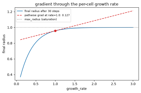
Because the rate lives in the state, the whole rollout is differentiable with respect to it: a morphology objective (here the final radius after a fixed time) has a well-defined gradient d(final radius) / d(growth_rate). This is exactly what lets an upstream controller that writes growth_rate be trained by backpropagating through growth. We sweep the rate and overlay the pathwise gradient jax.grad returns.

model = jxm.Model([SaturatingCellGrowth(max_radius=1.0)])
State = jxm.build_state_from_model(model)


@jax.jit
def final_radius(rate0):
    s = State.init_empty(capacity=1, n_space_dim=2, n_types=1)
    s = s.update(
        alive=s.alive.at[0].set(True),
        radius=s.radius.at[0].set(0.15),
        growth_rate=s.growth_rate.at[0].set(rate0),
    )
    return jxm.simulate(model, s, n_steps=30, dt=0.1).radius[0]


grad_final = jax.jit(jax.grad(final_radius))
rates = np.linspace(0.1, 3.0, 60)
vals = np.array([float(final_radius(jnp.array(r))) for r in rates])

r0 = 1.0
g0 = float(grad_final(jnp.array(r0)))
v0 = float(final_radius(jnp.array(r0)))
print('d(final radius) / d(growth_rate) at rate=1.0:', g0)

fig, ax = plt.subplots(figsize=(6, 4))
ax.plot(rates, vals, label='final radius after 30 steps')
ax.plot(rates, v0 + g0 * (rates - r0), '--', color='tab:red', label=f'pathwise grad at rate=1.0: {g0:.3f}')
ax.axhline(1.0, color='0.5', ls=':', label='max_radius (saturation)')
ax.scatter([r0], [v0], color='tab:red', zorder=5)
ax.set(xlabel='growth_rate', ylabel='final radius', title='gradient through the per-cell growth rate')
ax.legend(fontsize=8)
fig.tight_layout()
plt.show()

d(final radius) / d(growth_rate) at rate=1.0: 0.12695702433805273

6. Putting it together: a growing, relaxing cluster

The steps compose. A model of MechanicalRelaxation (quasistatic, on positions) and SaturatingCellGrowth (dynamic, on radii) writes disjoint fields, so each macro-step relaxes the packing at the current sizes and then grows the cells a little. As the radii grow, the contact distance sigma = r_i + r_j grows with them, so the relaxed cluster expands while staying mechanically packed.

pot = Morse()
model = jxm.Model(
    [MechanicalRelaxation(pot, max_steps=500, f_tol=1e-6), SaturatingCellGrowth(max_radius=0.9)]
)
State = jxm.build_state_from_model(model)

# A small, compact cluster of 14 cells on a lightly jittered grid (spacing 0.55 ~ contact for
# radius 0.25), so every cell is within the Morse range and the first relaxation packs it cleanly.
n = 14
gx, gy = np.meshgrid(np.arange(4), np.arange(4))
grid = 0.55 * np.stack([gx.ravel(), gy.ravel()], axis=1).astype(float)[:n]
grid = grid - grid.mean(0)
start = grid + 0.02 * np.asarray(jax.random.normal(jax.random.PRNGKey(5), (n, 2)))

s = State.init_empty(capacity=n, n_space_dim=2, n_types=1)
s = s.update(
    alive=s.alive.at[:].set(True),
    radius=s.radius.at[:].set(0.25),
    growth_rate=s.growth_rate.at[:].set(1.0),
    celltype=s.celltype.at[:, 0].set(1.0),
    position=s.position.at[:].set(start),
)
s_end = jxm.simulate(model, s, n_steps=14, dt=0.1)  # deterministic: relax + grow each macro-step

# Share the grown cluster's (larger) limits across both panels so the start really looks small.
xlim, ylim = shared_limits(s_end)

fig, (a0, a1) = plt.subplots(1, 2, figsize=(11, 5))
jxm.viz.draw(s, ax=a0, color='tab:green', alpha=0.45, lims=(xlim, ylim), title='start: small, packed')
jxm.viz.draw(s_end, ax=a1, color='tab:blue', alpha=0.45, lims=(xlim, ylim),
             title='grown + kept relaxed')
fig.tight_layout()
plt.show()

print('mean radius:', f'{float(s.radius.mean()):.3f} -> {float(s_end.radius.mean()):.3f}',
      '| cluster expands as the cells grow while staying in contact')

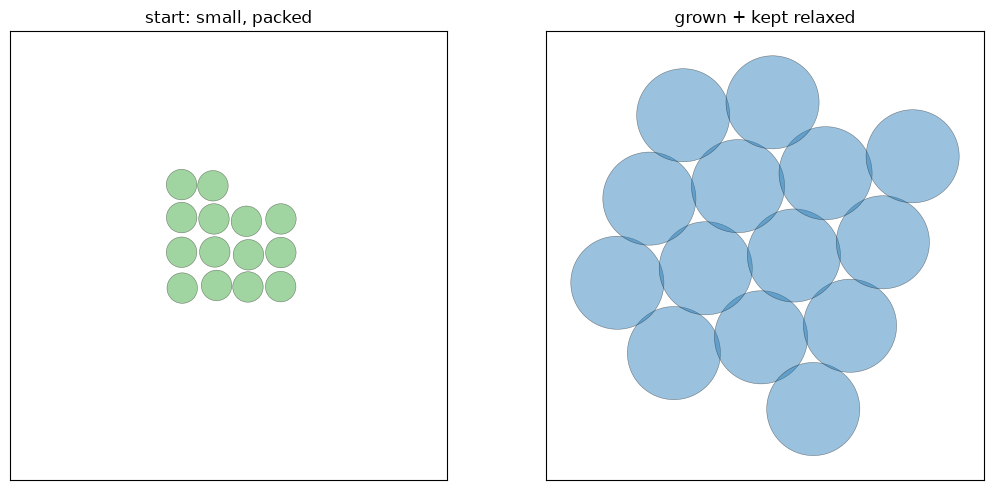
mean radius: 0.250 -> 0.763 | cluster expands as the cells grow while staying in contact